Maximum Heart Rate in Healthy and Unhealthy People
I. Introduction
Frequentist methods remain the prevailing form of statistics through which comparison of healthy and unhealthy patient groups is performed. It is the suite of statistical methods commonly taught to scientists and has historically come with the advantage of being simpler to enact and understand relative to Bayesian methods. With the growth of Bayesian computing in the last decade, however, this is no longer entirely the case. Setting up a comparative analysis of healthy and unhealthy patient groups is as simple as specifying some parameters for specific distributions that reflect the scientist’s own background knowledge on differences between healthy and unhealthy patient groups and using modern Markov Chain methods to approximate posterior distributions from which analysis can be performed. The workflow for how such a statistical comparative analysis might be performed is still opaque to many scientists, however.
A simple Bayesian comparative analysis of healthy and unhealthy patient groups involves setting two prior distributions related to sample physiologic measures in these two groups. Bayes’ theorem says that the prior distributions corresponding to each group can be updated with these samples of data to obtain posterior distributions related to these two groups’ physiologic measurements. This approach additionally comes with a theoretical guarantee of i.i.d within-group data that frequentist methods do not.
A Bayesian comparison of healthy and unhealthy subject groups is useful for performing more nuanced and detailed comparison of these two groups relative to frequentist approaches. To illustrate this process of Bayesian comparison of a physiologic measure between healthy and unhealthy groups, this paper implements a Bayesian analysis on a dataset with healthy subjects and subjects with heart disease. Subjects’ maximum heart rate is compared by forming prior distributions for the mean and standard deviation of each population’s maximum heart rate measures, obtaining posterior distributions for each of these statistics in the two groups, and using said posterior distributions to assess both groups.
II. Theoretical Framework
Let \(\theta_0\) and \(\sigma_0\) represent the mean and standard deviation of maximum heart rate among healthy people and \(\theta_1\) and \(\sigma_1\) represent the mean and standard deviation of maximum heart rate among people with heart disease. Also define \(n_0\) as the number of healthy subjects in a sample, \(n_1\) as the number of subjects with heart disease in a sample, \(y_{0i}\) as the maximum heart rate of a healthy sample patient, and \(y_{1j}\) as the maximum heart rate of a sample patient with heart disease, with \(i \in \{1,2,..., n_0\}\) and \(j \in \{1,2,..., n_1\}\). Also let \(k \in \{0,1\}\). Then we can define the joint likelihood probability distribution for each group as \[f(y_{k1},y_{k2},...,y_{kn_k}|\theta_k,\sigma_k^2)= \prod_{h=1}^{n_k}f(y_{kh}|\theta_k,\sigma_k)= \prod_{h=1}^{n_k}N(\theta_k,\sigma_k^2)\] Note that this assumes the within-group maximum heart rates are conditionally independently, identically distributed. Since each observation contains no other data besides maximum heart rate and heart disease status, observations that share the same disease status are treated as exchangeable. de Finetti’s theorem tells us they are thus independently, identically distributed given their distribution parameters are known. Also note that the likelihood for each observation \(y_{kh}\) is assumed to be \(N(\theta_k,\sigma_k^2)\). This is due to the general population of heart rates being known to have a normal distribution.
Now define the prior distribution for \(\theta_k\), or each group’s population mean, as \(f(\theta_k) = N(\mu_k, \tau_k)\) and the prior distribution for \(\sigma_k\), or each group’s population standard deviation, as \(f(\sigma_k) = Gamma(\alpha_k,\beta_k)\). In order to avoid making any assumptions about the relationship between \(\sigma_k\) and \(\theta_k\), their joint prior distribution is a product of their marginal prior distributions, or \[f(\theta_k,\sigma_k) = Gamma(\alpha_k,\beta_k)N(\mu_k, \tau_k)\] Bayes’ theorem thus tells us the posterior distribution is \[f(\theta_k,\sigma_k|y_{k1},y_{k2},...,y_{kn_k}) = \frac{f(y_{k1},y_{k2},...,y_{kn_k}|\theta_k,\sigma_k^2) f(\theta_k,\sigma_k)}{\iint_{A,B} f(y_{k1},y_{k2},...,y_{kn_k}|\theta_k,\sigma_k^2) f(\theta_k,\sigma_k) \, d\sigma_kd\theta_k}\] with \(A = (-\infty,\infty)\) and \(B=(0,\infty)\). This posterior distribution can be approximated through MC sampling. A posterior predictive probability of interest is also \(P(y_{1}^{*} > y_{0}^{*})\), in which \(y_1^*\) is a new observed maximum heart rate from the population of people with heart disease and \(y_0^*\) is a new observed maximum heart rate from a healthy population. This can be approximated through MCMC sampling.
III. Advantages of a Bayesian Comparative Analysis
A normal frequentist approach to assessing the difference in the maximum heart rates of these two populations would consist of calculating a t-statistic using the difference in the groups’ sample means and sample standard deviations and finding the p-value of this t-statistic given a t-distribution centered at 0. This p-value would be used to determine whether there is a difference between these groups’ mean maximum heart rate value or not given a cutoff value \(\delta\).
An issue with this approach is it does not allow for detailed comparison of any measure between two groups. The strict \(\delta\) cutoff makes it so there either is or is not a difference in the means of these two groups. This is problematic when issues of effect size or sampling variability are considered. What if there is a difference in the population means but one just happened to get a sample that suggests otherwise? What if there is a difference but the effect isn’t significant enough to allow this to be determined given the sample size used? In scenarios where we might still want to compare these groups despite the possibility of these scenarios occurring, a Bayesian approach allows for a more thorough assessment of these two groups relative to each other, instead of binding us to one of two assumptions. Furthermore, posterior distributions for these two groups can allow us to assess other statistics besides the mean, meaning a Bayesian approach allows for more detailed comparison of these two groups.
IV. Methodology
This was the workflow for this Bayesian analysis:
Choose likelihood distributions for the joint distributions of the samples in the two groups.
Decide on specific distributions for prior distributions and set parameters for them.
Perform a prior predictive check. This was done by sampling from the each group’s joint prior distribution and generating 1000 datasets for each group using the same likelihood function as the the group’s sample data and the same sample size as a specific group’s.This was followed by comparing the quantile of each group’s actual sample mean, sample median, and sample standard deviation to the generated datasets’ sample means, sample medians, and sample standard deviations.
Use a Markov Chain sampling technique to approximate samples from the posterior distributions. The NUTS algorithm was used for this project.
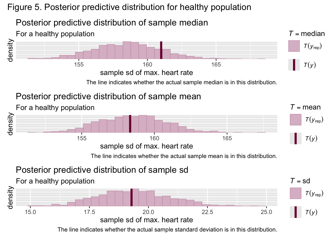
Perform a posterior predictive check with posterior samples using the same process outlined in step three.
Approximate the posterior predictive probability of a healthy person’s maximum heart rate being greater than a heart diseased person’s maximum heart rate by sampling from posterior distributions, generating one piece of data from each group, using an indicator function with the condition that the piece of data corresponding to the healthy group is greater than the piece of data corresponding to the unhealthy group, and calculating the mean of all these indicator function values.
V. Data Analysis
The dataset used for this analysis has 270 observations, with \(n_0 = 150\) and \(n_1 = 120\). Only the maximum heart rate and heart disease variables in it are considered in this analysis. The following questions are addressed through the following manners:
To what extent are the mean maximum heart rates and maximum heart rate standard deviations between healthy people and people with heart disease different? This is assessed through graphs of the posterior draws and the magnitude of their overlap areas.
What is the probability that a healthy person will have a greater maximum heart rate than a person with heart disease? This is assessed through the process outlined in step 6 of section 4.
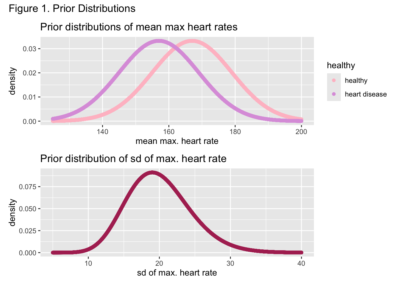
The following specifications for the standard deviation priors were made: \(\alpha_0 = \alpha_1 = 20\) and \(\beta_0 = \beta_1 = 1\). The parameters for the prior of the heart disease population mean were specified as \(\mu_1 = 157\) and \(\tau_1 = 12\), while the parameters for the prior of the healthy population were specified as \(\mu_0 = 167\) and \(\tau_0 = 12\). These decisions were based on the commonly known manner for calculating maximum heart rate, \(220 - age\). Since the sample consisted of all adults, the mean priors approximately cover \((220-79,220-18)\), reflected in Figure 1. Similarly, given this large range of adult maximum heart rates, it was assumed the population standard deviations for both groups was at minimum approximately \(10\) and at maximum approximately \(30\), which the shared gamma prior in Figure 1 for both populations reflects. \(\mu_1\) is smaller than \(\mu_0\) to reflect knowledge in the literature about the reduced heart rate capabilities of people with heart disease.
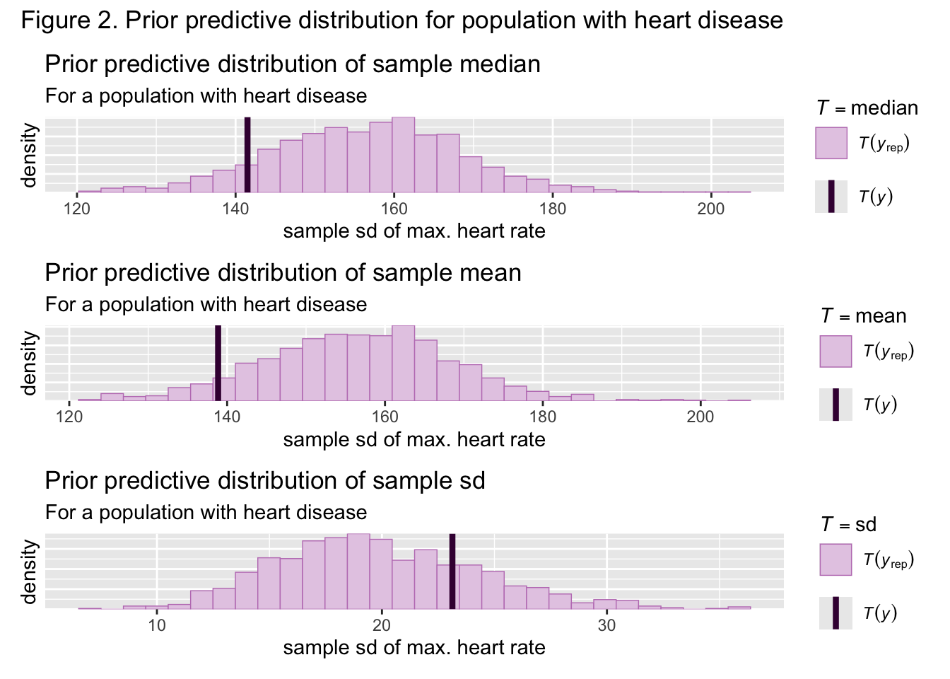
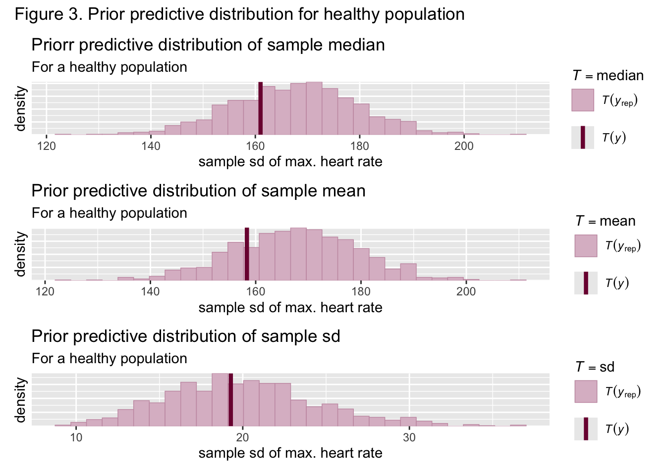
Figures 2 and 3 show the sample mean, median, and standard deviation for both groups was nestled well within the bounds of the generated prior predictive sample means, medians, and standard deviations, meaning that the priors are suited to the data. Samples from both the healthy and unhealthy posterior distributions were then approximated through the NUTS algorithm. Figures 4 and 5 show that the actual sample means, medians, and standard deviations are nestled well within the bounds of the generated posterior predictive statistics, implying the posterior is also suited to this data
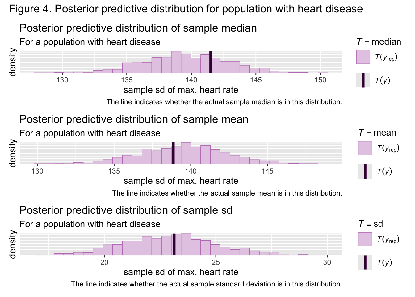
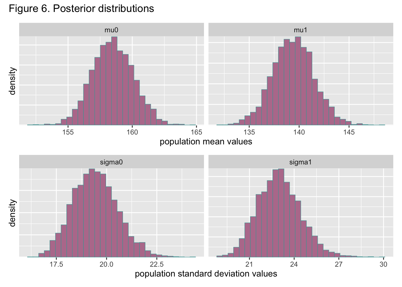
Based on figure 6, the maximum heart rate means of both populations are different by at least 10. Figure 4 also shows a little overlap between the distributions of both population standard deviations but not much. Overall, the difference in the distributions of population standard deviations is a lot less pronounced than the difference in the distributions of population means, although there is still a major difference. Based on the calculation outlined in step 6 of section 4, the probability of any healthy subject having a maximum heart rate greater than that of someone with heart disease is approximately 1, meaning it is extremely likely this will be the case. These results indicate that the maximum heart rate of the typical healthy person is higher than the maximum heart rate of a typical person with heart disease, which follows trends in the literature on heart rate.
VI. Conclusion
This paper demonstrates a Bayesian approach to a comparative analysis of healthy and heart disease groups. The results follow trends in the literature about heart rate capability in healthy and unhealthy people. Further comparison of these populations could be made through posterior predictive calculations of other measures as well. Overall, this paper represents a simple workflow through which comparison of healthy and unhealthy groups can be performed.