library(RTextTools)
library(tidyverse)
library(tidytuesdayR)Netflix
Introduction
This project consists of me analyzing data about Netflix shows and movies, with said analysis focusing on two aspects of these: horror movies and number of seasons in said shows. The dataset used for this analysis can be found here. According to the Tidy Tuesday github page I found it in, it originates from Kaggle and was gathered by Shival Bansal. Here is what he says about the data:
This dataset consists of tv shows and movies available on Netflix as of 2019. The dataset is collected from Flixable which is a third-party Netflix search engine.
In 2018, they released an interesting report which shows that the number of TV shows on Netflix has nearly tripled since 2010. The streaming service’s number of movies has decreased by more than 2,000 titles since 2010, while its number of TV shows has nearly tripled. It will be interesting to explore what all other insights can be obtained from the same dataset.
Here is the data dictionary (sourced from here): d | variable | class | description | |:—————-|:—————-|:————————————-| | show_id | character | Unique ID for every Movie / Tv Show | | type | character | Identifier - A Movie or TV Show | | title | character | Title of the Movie / Tv Show | | director | character | Director of the Movie/Show | | cast | character | Actors involved in the movie / show | | country | character | Country where the movie / show was produced | | date_added | character | Date it was added on Netflix | | release_year | double | Actual Release year of the movie / show | | rating | character | TV Rating of the movie / show | | duration | character | Total Duration - in minutes or number of seasons | | listed_in | character | Genre | | description | character | Summary description of the film/show |
netflix <- readr::read_csv('https://raw.githubusercontent.com/rfordatascience/tidytuesday/main/data/2021/2021-04-20/netflix_titles.csv')Netflix Horror Movies
In this analysis of Netflix horror movies, I look at all movies with horror listed as a genre and see what other genres are also listed for said movies. I then create a bar plot comparing the number of other genres listed among Netflix horror movies.
First, I filter for movies with horror listed as one of its genres and clean the variable listing movie genres so that it only includes genres that aren’t horror. This is all saved in the “horror_subgenre” object.
horror_subgenre <- netflix %>%
  filter(str_detect(listed_in, "Horror"), type == "Movie") %>%
  mutate(listed_in = str_remove(listed_in, ", International Movies")) %>%
  mutate(listed_in = str_remove(listed_in, ", Independent Movies")) %>%
  mutate(listed_in = str_remove_all(listed_in, "[,]")) %>%
  mutate(listed_in = str_remove_all(listed_in, "Movies")) %>%
  mutate(listed_in = str_replace(listed_in, "[:space:]&[:space:]", "&")) %>%
  group_by(listed_in) %>%
  summarize(num = n()) %>%
  arrange(desc(num)) %>%
  mutate(listed_in = str_remove(listed_in, "Horror"))
Then, I count the number of movies within “horror_subgenre” that list a specific secondary genre, with the secondary genres I consider being the following: thriller, comedy, romance, action/adventure, science fiction and fantasy, cult, documentary, and none. None means that the movie only has horror as its genre.
num_thrillers <- horror_subgenre %>%
  group_by(str_detect(listed_in,"Thrillers")) %>%
  summarize(num = sum(num)) %>%
  rename(Thrillers = 'str_detect(listed_in, \"Thrillers\")') %>%
  filter(Thrillers == TRUE) %>%
  mutate(genre = "Thrillers") %>%
  select(-Thrillers)

num_comedies <- horror_subgenre %>%
  group_by(str_detect(listed_in,"Comedies")) %>%
  summarize(num = sum(num)) %>%
  rename(Comedies = 'str_detect(listed_in, \"Comedies\")') %>%
  filter(Comedies == TRUE) %>%
  mutate(genre = "Comedies") %>%
  select(-Comedies)


num_action_adventure <- horror_subgenre %>%
  group_by(str_detect(listed_in,"Action/Adventure"))%>%
  summarize(num = sum(num)) %>%
  rename(Action_Adventure = 'str_detect(listed_in, \"Action/Adventure\")') %>%
  filter(Action_Adventure == TRUE) %>%
  mutate(genre = "Action&Adventure") %>%
  select(-Action_Adventure)

num_scifi_fantasy <- horror_subgenre %>%
  group_by(str_detect(listed_in,"Sci-Fi&Fantasy")) %>%
  summarize(num = sum(num)) %>%
  rename(SciFi_Fantasy = 'str_detect(listed_in, \"Sci-Fi&Fantasy\")') %>%
  filter(SciFi_Fantasy == TRUE) %>%
  mutate(genre = "SciFi&Fantasy") %>%
  select(-SciFi_Fantasy)

num_cult <- horror_subgenre %>%
  group_by(str_detect(listed_in,"Cult")) %>%
  summarize(num = sum(num)) %>%
  rename(Cult = 'str_detect(listed_in, \"Cult\")') %>%
  filter(Cult == TRUE) %>%
  mutate(genre = "Cult") %>%
  select(-Cult)

num_documentaries <- horror_subgenre %>%
  group_by(str_detect(listed_in,"Documentaries")) %>%
  summarize(num = sum(num)) %>%
  rename(Documentaries = 'str_detect(listed_in, \"Documentaries\")') %>%
  filter(Documentaries == TRUE)%>%
  mutate(genre = "Documentaries") %>%
  select(-Documentaries)

num_romantic <- horror_subgenre %>%
  group_by(str_detect(listed_in,"Romantic")) %>%
  summarize(num = sum(num)) %>%
  rename(Romantic = 'str_detect(listed_in, \"Romantic\")') %>%
  filter(Romantic == TRUE) %>%
  mutate(genre = "Romantic") %>%
  select(-Romantic)

num_horror <- horror_subgenre %>%
  filter(listed_in == " ") %>%
  mutate(listed_in = "none") %>%
  rename(genre = listed_in) %>%
  select(genre, num)

horror_df <- rbind(num_thrillers, num_comedies, num_action_adventure, num_scifi_fantasy, num_cult, num_documentaries, num_romantic, num_horror ) %>%
  as.data.frame() %>%
  arrange(desc(num)) %>%
  select(genre, num)
horror_df
genre num
1 none 125
2 Thrillers 110
3 Comedies 38
4 SciFi&Fantasy 19
5 Cult 12
6 Documentaries 2
7 Romantic 2ggplot(horror_df, aes(x = genre, y = num)) +
geom_bar(stat = "identity", aes(fill = genre)) + labs(
title = "Subgenres among netflix horror movies",
x = "Subgenre of horror movie",
y = "Count"
) +
scale_x_discrete(guide = guide_axis(n.dodge=3)) +
guides(fill=guide_legend(title="Subgenres"))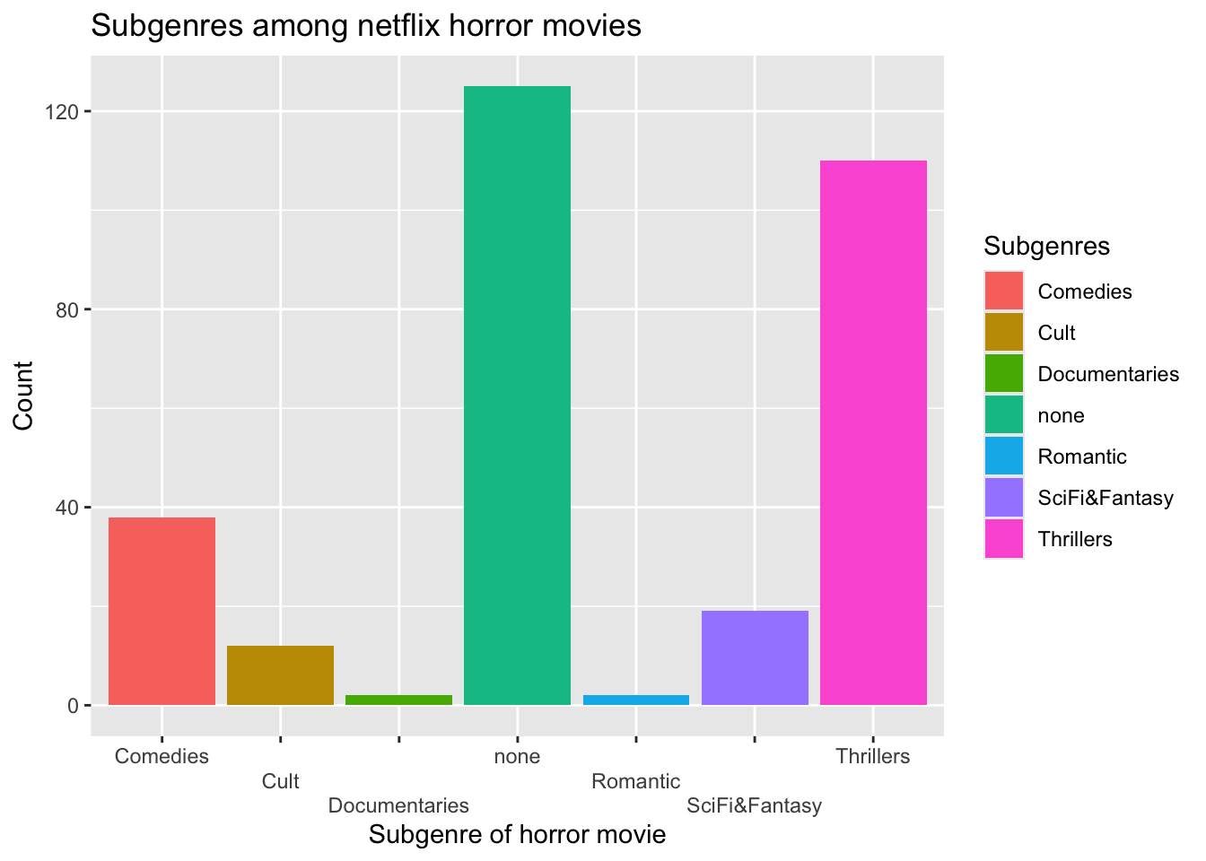
Based on this plot of the number of horror movies with specific secondary genres, it seems most netflix horror movies either do not have a secondary genre or have thriller as their secondary genre. Other secondary genres appear less present among Netflix horror movies.
Netflix TV Shows
In this analysis of Netflix tv shows, I look at the number of seasons present in Netflix shows released in different years. A season in a Netflix show is a set of episodes pertaining to said show that was greenlit to be released in a certain time period. A show having multiple seasons means different sets of episodes were allowed to be released at different periods of time.
data <- netflix %>%
  filter(type == "TV Show") %>%
  mutate(num_seasons = as.numeric(str_extract(duration, "\\d+" )))

ggplot(data, aes(x = release_year, y = num_seasons)) +
  geom_point() +
  xlim(1970,2025)+
  geom_smooth(se = FALSE) +
  labs(
    title = "Relationship between release year and number of seasons of netflix tv show",
    x = "Release year",
    y = "Number of seasons"
  )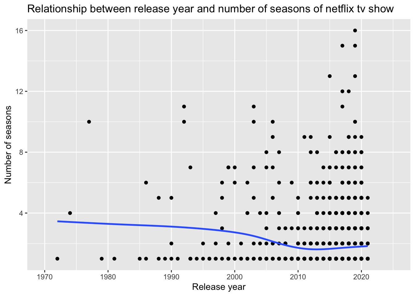
Based on this plot, the number of seasons that a Netflix show has tends to be lower for shows released between 2005 and 2020 than for other shows. Due to the discreteness of values on the x-axis, multiple points are most likely overlapping. This explains why it appears the right side of the graph has less points below the line of best fit than above it even with the line trending downwards.
Data source here.